Motion Given by a Motion Graph II
Task number: 1747
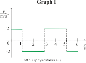
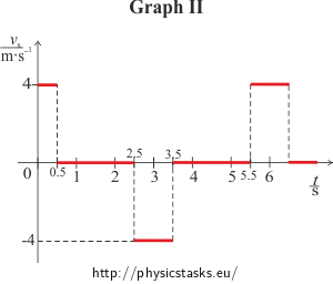
There are two graphs shown in the pictures.
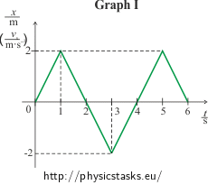
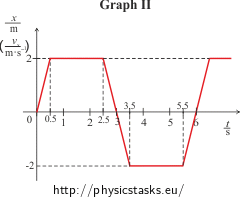
a) Consider them to be position-time graphs of uniform linear motions and chart the corresponding speed-time graphs.
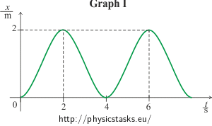
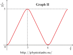
b) Consider them to be speed-time graphs of uniform linear motions and chart the corresponding position-time graphs.
Do the graphs represent real motions? Try to trace the motions with your finger.
Hint 1 for a): Dividing the graphs into intervals
Consider the graphs to be visual representations of functions x(t), where x(t) is the time dependence of x.
Divide the graphs into separate time intervals.
How does the position change in time? Express it with equations.
Hint 2 for a): Describing the motions
Use the equations for x(t) from previous hint to determine the equations for vx(t) for each interval and plot the graphs of functions vx(t) over these intervals.
What motion do the equations represent?
Hint 3 for a): Realism of the motion
Try to trace the motions with your finger. Is it possible to suddenly change the speed as shown in the graph?
Hint 4 for b): Dividing the graphs into intervals
Consider the graphs to be visual representations of functions vx(t), where vx(t) is the time dependence of v.
Follow the same steps as in Hint 1 and 2 for a):
Divide the graphs into intervals. What functions do the segments of the graphs represent? Write down the corresponding equations.
Hint 5 for b): Describing the motions
Use the equations for vx(t) from previous hint to determine the equations for x(t) for each interval and plot the graphs of functions x(t) over these intervals.
What motion do the equations represent?
Hint 6 for b): Realism of the motion
Try to trace the motions with your finger.
COMPLETE SOLUTION
Ad a):
We consider the graphs to be visual representations of functions x(t), where x(t) is the time dependence of x.
We divide the graphs into separate time intervals.
We find the equations that represent the functions over individual intervals.
Note: An example of a distance-time dependence written in the form of an equation is:
x(t) = 2 m·s−1t +1m.
We won’t write the units to make the notation simpler.
For graph I we get the following intervals:
<0 s; 1 s> The function is a line x(t) = 2t (the position increases uniformly),
(1 s; 3 s> The function is a line x(t) = −2t + 4 (the position decreases uniformly),
(3 s; 5 s> The function is a line x(t) = 2t − 8 (the position increases uniformly),
(5 s; 6 s> The function is a line x(t) = −2t + 12 (the position decreases uniformly).
For graph II we get the following intervals:
<0 s; 0.5 s> The function is a line x(t) = 4t (the position increases uniformly),
(0.5 s; 2.5 s> The function is a line x(t) = 2 (the position doesn’t change),
(2.5 s; 3.5 s> The function is a line x(t) = −4t + 12 (the position decreases uniformly).
(3.5 s; 5.5 s> The function is a line x(t) = −2 (the position doesn’t change),
(5.5 s; 6.5 s> The function is a line x(t) = 4t − 24 (the position increases uniformly),
(6.5 s; 8.5 s> The function is a line x(t) = 2 (the position doesn’t change).
We use the equations for x(t) to determine the equations for vx(t) for each interval and plot the graphs of functions vx(t) over these intervals.
We get the time dependence of speed vx(t) by differentiating the time dependence of position x(t).
Graph I:
For the interval <0 s; 1 s>:
\[v_x(t) = \frac{\mathrm{d}x(t)}{\mathrm{d}t} = \frac{d(2t)}{\mathrm{d}t} = 2.\]
The object is in a uniform linear motion with constant speed of 2 m·s−1 in the direction of the x axis.
For the interval (1 s; 3 s>:
\[v_x(t)\,=\,\frac{\mathrm{d}x(t)}{\mathrm{d}t} \,=\, \frac{d(-2t + 4)}{\mathrm{d}t} \,= -2.\]
The object is in a uniform linear motion with constant speed of 2 m·s−1 against the direction of the x axis.
For the interval (3 s; 5 s>:
\[v_x(t) \,=\, \frac{\mathrm{d}x(t)}{\mathrm{d}t} \,=\, \frac{d(2t - 8)}{\mathrm{d}t} \,=\, 2.\]
The object is in a uniform linear motion with constant speed of 2 m·s−1 in the direction of the x axis.
For the interval (5 s; 6 s>:
\[v_x(t) \,=\, \frac{\mathrm{d}x(t)}{\mathrm{d}t} \,=\, \frac{d(-2t + 12)}{\mathrm{d}t} \,=\, -2.\]
The object is in a uniform linear motion with constant speed of 2 m·s−1 against the direction of the x axis.
Graph II:
For the interval <0 s; 0.5 s>:
\[v_x(t) \,=\, \frac{\mathrm{d}x(t)}{\mathrm{d}t} \,=\, \frac{d(4t)}{\mathrm{d}t} \,=\, 4.\]
The object is in a uniform linear motion with constant speed of 4 m·s−1 in the direction of the x axis.
For the interval (0.5 s; 2.5 s>:
\[v_x(t) \,=\, \frac{\mathrm{d}x(t)}{\mathrm{d}t} \,=\, \frac{d(2)}{\mathrm{d}t} \,=\, 0.\]
The object doesn’t move, it is at rest (vx = 0 m·s−1).
For the interval (2.5 s; 3.5 s>:
\[v_x(t) \,=\, \frac{\mathrm{d}x(t)}{\mathrm{d}t} \,=\, \frac{d(-4t + 12)}{\mathrm{d}t} \,=\, -4.\]
The object is in a uniform linear motion with constant speed of 4 m·s−1 against the direction of the x axis.
For the interval (3.5 s; 5.5 s>:
\[v_x(t) \,=\, \frac{\mathrm{d}x(t)}{\mathrm{d}t} \,=\, \frac{d(-2)}{\mathrm{d}t} \,=\, 0.\]
The object doesn’t move, it is at rest (vx = 0 m·s−1).
For the interval (5.5 s; 6.5 s>:
\[v_x(t) \,=\, \frac{\mathrm{d}x(t)}{\mathrm{d}t} \,=\, \frac{d(4t - 24)}{\mathrm{d}t} \,=\, 4.\]
The object is in a uniform linear motion with constant speed of 4 m·s−1 in the direction of the x axis.
For the interval (6.5 s; 8.5 s>:
\[v_x(t) \,=\, \frac{\mathrm{d}x(t)}{\mathrm{d}t} \,=\, \frac{\mathrm{d}(2)}{\mathrm{d}t} \,=\, 0.\]
The object doesn’t move, it is at rest (vx = 0 m·s−1).
These are not realistic motions.
The speed of a real motion cannot change suddenly. When tracing the motion with your finger, it must first slow down to zero speed and then start moving in the other direction. A position-time graph of such motion would not include sharp peaks.
Ad b):
We follow the same steps as in part a).
Note: Again, we won’t write the units to make the notation simpler.
We consider the graphs to be visual representations of functions vx(t), where vx(t) is the time dependence of v.
We divide the graphs into intervals. We write down the functions that represent the motions on these intervals.
Graph I:
<0 s; 1 s> the function is a line vx(t) = 2t,
(1 s; 3 s> the function is a line vx(t) = −2t + 4,
(3 s; 5 s> the function is a line vx(t) = 2t − 8,
(5 s; 6 s> the function is a line vx(t) = −2t + 12.
Graph II:
<0 s; 0,5 s> the function is a line vx(t) = 4t,
(0.5 s; 2.5 s> the function is a line vx(t) = 2,
(2.5 s; 3.5 s> the function is a line vx(t) = −4t + 12,
(3.5 s; 5.5 s> the function is a line vx(t) = −2,
(5.5 s; 6.5 s> the function is a line vx(t) = 4t − 24,
(6.5 s; 8.5 s> the function is a line vx(t) = 2.
We use the equations for vx(t) to determine the equations for x(t) for each interval and plot the graphs of functions x(t) over these intervals.
We get the time dependence of position x(t) by integrating the time dependence of speed vx(t).
Note: Again, we won’t write the units to make the notation simpler.
Graph I:
For interval <0 s; 1 s>:
\[x(t)\,=\,\int{v_x(t)}\mathrm{d}t\,=\,\int{2t}\mathrm{d}t,\]
\[x(t)\,=\, t^{2}+A.\]
The constant of integration A can be calculated from the initial conditions:
The position at time t = 0 s is x(0) = 0 m, therefore A = 0.
\[x(t) \,=\, t^{2}.\]
The object is in a uniformly accelerated linear motion in the direction of the x axis.
For interval (1 s; 3 s>:
\[x(t) \,=\, \int{v_x(t)}\mathrm{d}t\,=\,\int{(-2t+4)}\mathrm{d}t,\]
\[x(t) \,=\, -t^{2}+4t+B.\]
The constant of integration B can be calculated from the initial conditions:
We will calculate the position at time t = 1 s by evaluating the previous equation \(x(t)\,=\,t^{2}\), we get x(1) = 1 m.
We substitute into the equation: 1 = −12 + 4·1 + B, therefore B = −2.
\(x(t) \,=\, -t^{2}+4t-2\)
The object is in a uniformly decelerated linear motion in the direction of the x axis. At time t = 2 s the speed is zero, the direction of the motion reverses and the object moves in a uniformly accelerated linear motion against the direction of the x axis.
For interval (3 s; 5 s>:
\[x(t) \,=\, \int{v_x(t)}\mathrm{d}t\,=\,\int{(2t-8)}\mathrm{d}t,\]
\[x(t) \,=\, t^{2}-8t+C.\]
The constant of integration C can be calculated from the initial conditions:
We will calculate the position at time t = 3 s by evaluating the previous equation \(x(t)\,=\,-t^{2}+4t-2\), we get x(3) = 1 m.
We substitute into the equation: 1 = 32−8·3 + C, therefore C = 16.
\(x(t)\,=\,t^{2}-8t+16\)
The object is in a uniformly decelerated linear motion against the direction of the x axis. At time t = 4 s the speed is zero, the direction of the motion reverses and the object moves in a uniformly accelerated linear motion in direction of the x axis.
For interval (5 s; 6 s>:
\[x(t) \,=\, \int{v_x(t)}\mathrm{d}t\,=\,\int{(-2t+12)}\mathrm{d}t,\]
\[x(t)\,=\,-t^{2}+12t+D.\]
The constant of integration D can be calculated from the initial conditions:
We will calculate the position at time t = 5 s by evaluating the previous equation \(x\,=\,t^{2}-8t+16\), we get x(5) = 1 m.
We substitute into the equation: 1 = −52+12·5 + D, therefore D = −34.
\(x(t) \,=\, -t^{2}+12t-34\)
The object is in a uniformly decelerated linear motion in the direction of the x axis.
Graph II:
For interval <0 s; 0.5 s>:
\[x(t) \,=\, \int{v_x(t)}\mathrm{d}t\,=\,\int{4t}\mathrm{d}t,\]
\[x(t) \,=\, 2t^{2}+E.\]
The constant of integration E can be calculated from the initial conditions:
The position at time t = 0 s is x(0) = 0 m, therefore E = 0.
\(x(t) \,=\, 2t^{2}\)
The object is in a uniformly accelerated linear motion in the direction of the x axis.
For interval (0.5 s; 2.5 s>:
\[x(t) \,=\, \int{v_x(t)}\mathrm{d}t\,=\,\int{2}\mathrm{d}t,\]
\[x(t) \,=\, 2t+F. \]
The constant of integration F can be calculated from the initial conditions:
We will calculate the position at time t = 0.5 s by evaluating the previous equation \(x(t)\,=\,2t^{2}\), we get x(0.5) = 0.5 m.
We substitute into the equation: 0.5 = 2·0.5+F, therefore F = −0.5.
\(x(t) \,=\, 2t-0.5\)
The object is in a uniform linear motion at the speed of 2 m·s−1 in the direction of the x axis.
For interval (2.5 s; 3.5 s>:
\[x(t) \,=\, \int{v_x(t)}\mathrm{d}t\,=\,\int{(-4t+12)}\mathrm{d}t,\]
\[x(t) \,=\, -2t^{2}+12t+G.\]
The constant of integration G can be calculated from the initial conditions:
We will calculate the position at time t = 2,5 s by evaluating the previous equation \(x(t)\,=\,2t-0.5\), we get x(2.5) = 4.5 m.
We substitute into the equation: 4.5 = −2·2.52 + 12·2.5 + G, therefore G = −13.
\(x(t) \,=\, -2t^{2}+12t-13\)
The object is in a uniformly decelerated linear motion in the direction of the x axis. At time t = 3 s the speed is zero, the direction of the motion reverses and the object moves in a uniformly accelerated linear motion against the direction of the x axis.
For interval (3.5 s; 5.5 s>:
\[x(t) \,=\, \int{v_x(t)}\mathrm{d}t\,=\,\int{-2}\mathrm{d}t,\]
\[x(t) \,=\, -2t+H. \]
The constant of integration H can be calculated from the initial conditions:
We will calculate the position at time t = 3.5 s by evaluating the previous equation \(x(t)\,=\,-2t^{2}+12t-13\), we get x(3.5) = 4.5 m.
We substitute into the equation:: 4.5 = −2·3.5 + H, therefore H = 11.5.
\(x(t) \,=\, -2t+11.5 \)
The object is in a uniform linear motion at the speed of 2 m·s−1 against the direction of the x axis.
For interval (5.5 s; 6.5 s>:
\[x(t) \,=\, \int{v_x(t)}\mathrm{d}t\,=\,\int{(4t-24)}\mathrm{d}t,\]
\[x(t) \,=\, 2t^{2}-24t+K.\]
The constant of integration K can be calculated from the initial conditions:
We will calculate the position at time t = 5.5 s by evaluating the previous equation \(x(t)\,=\,-2t+11.5 \), we get x(5.5) = 0.5 m.
We substitute into the equation: 0.5 = 2·5.52−24·5.5 + K, therefore K = 72.
\(x(t) \,=\, 2t^{2}-24t+72\)
The object is in a uniformly decelerated linear motion against the direction of the x axis. At time t = 6 s the speed is zero, the direction of the motion reverses and the object moves in a uniformly accelerated linear motion in the direction of the x axis.
For interval (6.5 s; 8.5 s>:
\[x(t) \,=\, \int{v_x(t)}\mathrm{d}t\,=\,\int{2}\mathrm{d}t,\]
\[x(t) \,=\, 2t+L. \]
The constant of integration L can be calculated from the initial conditions:
We will calculate the position at time t = 6.5 s by evaluating the previous equation \(x(t)\,=\,2t^{2}-24t+72\), we get x(6.5) = 0.5 m.
We substitute into the equation: 0.5 = 2·6.5 + L, therefore L = −12.5.
\(x(t) \,=\, 2t-12.5 \)
The object is in a uniform linear motion at the speed of 2 m·s−1 in the direction of the x axis.
The motions are realistic.
Graph I:Let’s say the finger starts moving to the right and for 1 s it accelerates uniformly and then decelerates uniformly for 1 s. At time t = 2 s the speed of the finger is equal to zero and the direction of the motion reverses. The finger moves to the left, it accelerates uniformly for 1 s then it decelerates uniformly for 1 s. At time t = 4 s the finger is at the same spot where the movement has originally started, the speed of the finger is zero and the motion repeats.
Graf II:Let’s say the finger starts moving to the right and for 0.5 s it accelerates uniformly and then moves with constant speed for 2 s. It then decelerates uniformly for 0.5 s until it reaches zero speed. That’s when the direction of the motion reverses and the finger starts moving to the left accelerating uniformly for 0.5 s. The finger then keeps moving with constant speed for 2 s and then decelerates uniformly for 0.5 s. The finger is then at the same spot where the movement has started, the speed of the finger is zero and the motion repeats.
Answer
